A photonic crystal guides light with a pattern that repeats on the scale of its wavelength. Stack two of them and twist one slightly, and a moiré pattern appears: a slow change in how the two layers line up, many times larger than either crystal. Twisted crystals like these can slow, trap, and reshape light.
They are also hard to describe and expensive to compute. At most angles the combined structure never repeats, and where it does, the repeating cell is so large that direct solvers run out of memory. My master’s thesis develops a two-scale theory that avoids this calculation: many small crystal calculations and one small problem for the slow pattern replace a single huge one.
Two scales from one twist
Each layer repeats with a spacing a. The twist adds a second, much larger period, the moiré period L = a / (2 sin(θ/2)): a twist of 2° already gives L ≈ 29a. Turn the angle below and watch the two scales separate. The moiré cell marks a repeating pattern of local alignment, not an exact repeat of the structure itself.
- Spacing a
- 1
- Period L/a
- 11.46
- Ratio η
- 0.087
Too large to compute directly
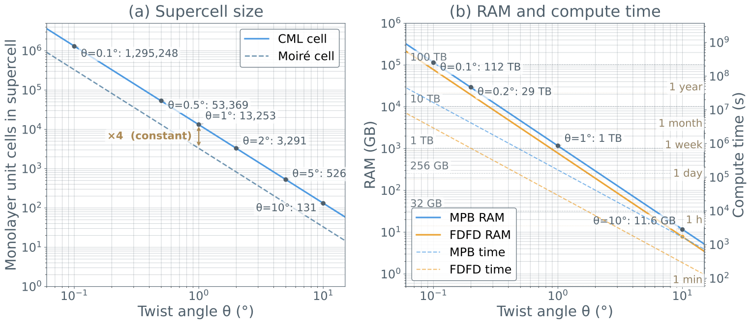
Solvers for periodic structures need a cell that repeats exactly. At a generic twist there is none; at special angles there is one, but it grows roughly as 1/θ² as the angle shrinks.
In the thesis, a full reference calculation at 2.01° needed about 3.3 million unknowns and about 54 minutes. The next such cell, at 1.01°, needed about 13 million and no longer fit in memory, just where the interesting physics begins.
A crystal that changes slowly
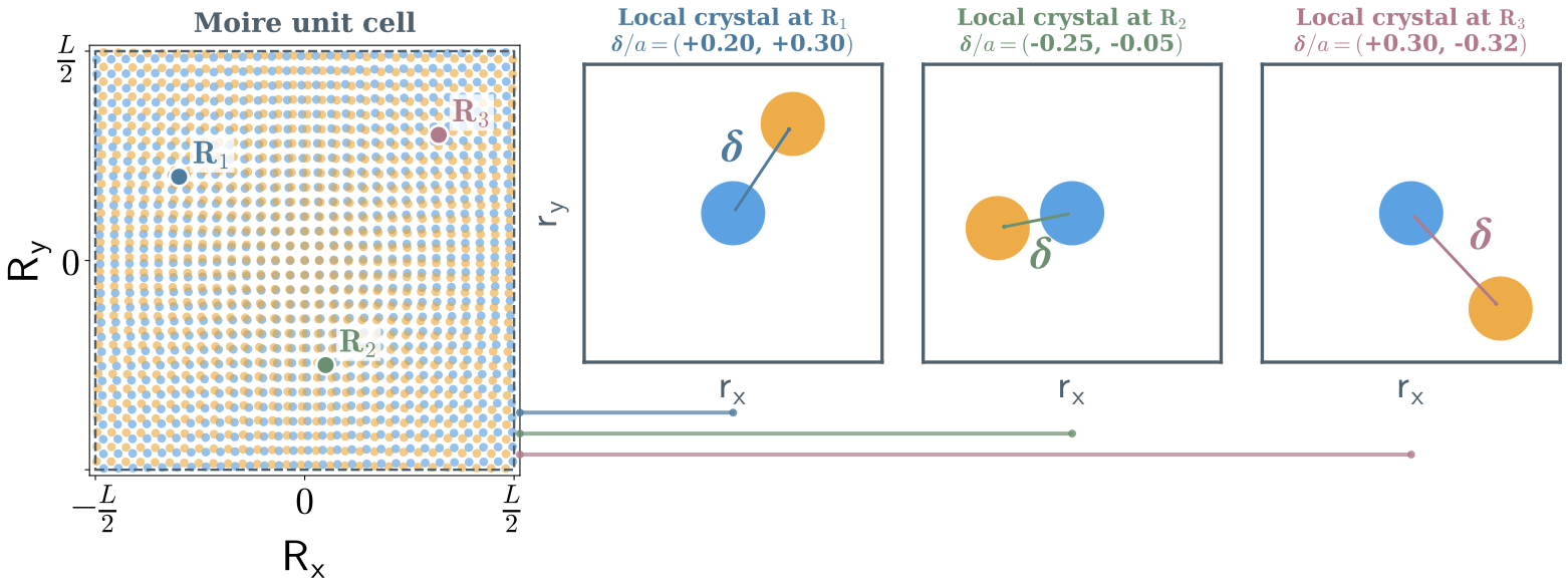
Seen up close, a slightly twisted bilayer looks like an ordinary crystal whose two layers are shifted against each other. That shift, the registry, changes slowly across the moiré cell. So the light can be written as the local crystal’s wave patterns, carried by a slow envelope that varies only on the moiré scale.
Only a few bands are kept, and the small ratio of the two scales, η, becomes the parameter of an expansion. The envelope then obeys an equation of its own, a far smaller problem to solve.
An equation for the envelope
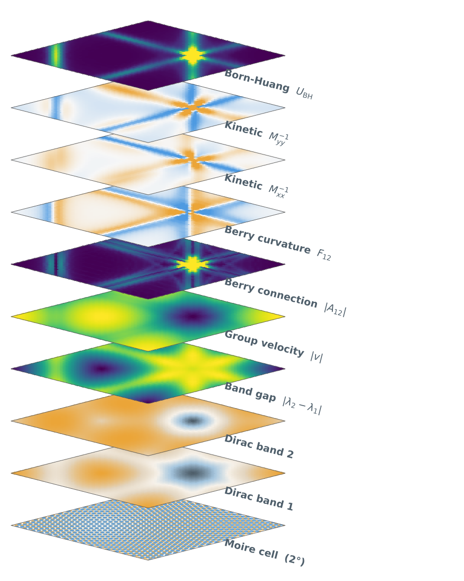
Projecting Maxwell’s equations onto the local wave patterns gives an effective Hamiltonian for the envelope, for both polarizations of light, TE and TM. Each term has a plain meaning: the local band energies, how fast the waves travel and how their bands curve, the Berry connection that tracks how the local patterns change with the registry, and corrections from the bands that were left out.
All coefficients are computed once per crystal and reused for every twist angle. The two cards open the full equations, term by term.
Why this needed Blaze2D
Assembling the equation needs more than just a high volume of band diagrams: at every registry point it requires the local wave patterns, their velocities and curvatures, and the couplings to the bands left out. Keeping four bands can mean solving sixteen or more, for thousands of slightly different crystals.
MPB, the standard solver, did not provide these quantities as the dataset the theory needed, so I built Blaze2D to compute them. The MSL pipeline assembles and solves the envelope problem from its output.
Tested against full calculations
The results here come from the second edition of the thesis, revised after submission: it corrects the derivation and rebuilds the validation as a comparison against two independent full-Maxwell solvers, one with plane waves and one on a spatial grid.
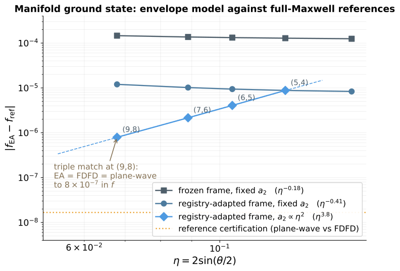
On a smooth, weakly coupled crystal, letting the local patterns follow the registry lowers the error about fifteenfold. When the second layer weakens along with the angle, the error falls with nearly the fourth power of η (a fitted exponent of 3.8), down to 8 × 10⁻⁷ in frequency against both references.
Every state accounted for
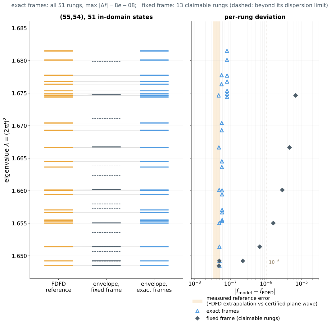
Similar-looking bands can hide missing or extra states, so the test matches every state in a window chosen in advance. At 0.607°, where one supercell holds 8,911 crystal cells, the model reproduces all 51 states in its window, with frequency differences of 4.7 × 10⁻⁸ to 8.1 × 10⁻⁸, comparable to the reference’s own numerical error.
What remains open
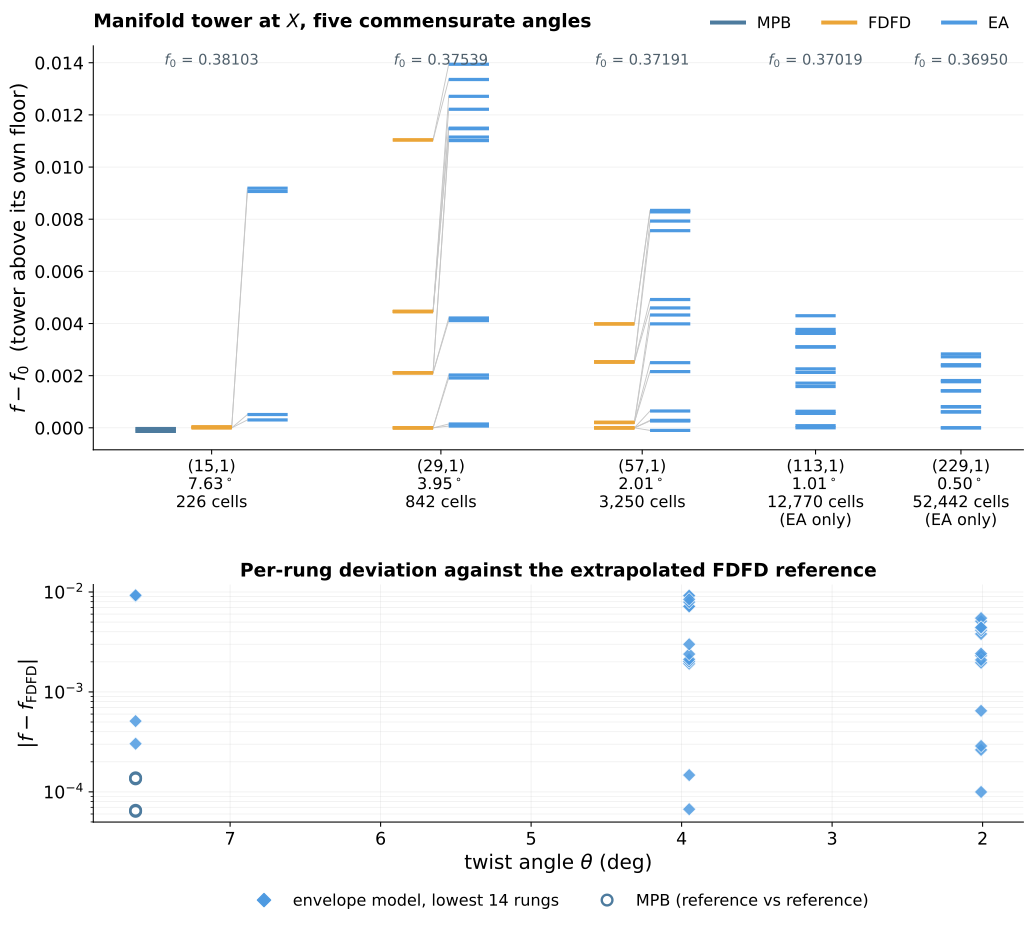
A square bilayer of rods is harder: its registry creates deep wells that trap the envelope. There the model brings the lowest state close to the references and reaches 0.50°, where the full calculation did not fit in memory. Higher up, groups of four states that symmetry says must share a frequency come out split.
Three steps remain: a symmetry-respecting gauge for the local patterns, the next order of the theory, and photonic slabs, the thin patterned films most experiments use. Slabs are also on Blaze’s roadmap.
Context
Primary references
- Bistritzer & MacDonald (2011): Moiré bands in twisted double-layer graphene
- Lopes dos Santos, Peres & Castro Neto (2007): Graphene bilayer with a twist: electronic structure
- Wang et al. (2020): Localization and delocalization of light in photonic moiré lattices
- Tang et al. (2021): Modeling the optical properties of twisted bilayer photonic crystals
- Lou et al. (2021): Theory for twisted bilayer photonic crystal slabs
- Yi, Park & Park (2022): Strong interlayer coupling and stable topological flat bands in twisted bilayer photonic moiré superlattices
- Huang, Zhang & Zhang (2022): Moiré quasibound states in the continuum
- Tang et al. (2023): Experimental probe of twist angle–dependent band structure of on-chip optical bilayer photonic crystal
- Du, Dai & Sun (2023): Moiré photonics and optoelectronics
- Oudich et al. (2024): Engineered moiré photonic and phononic superlattices
- Qin et al. (2024): Optical moiré bound states in the continuum
- Yan et al. (2025): Cavity quantum electrodynamics with moiré photonic crystal nanocavity
- Joannopoulos, Johnson, Winn & Meade (2008): Photonic Crystals: Molding the Flow of Light (2nd ed.)
- Johnson & Joannopoulos (2001): Block-iterative frequency-domain methods for Maxwell’s equations in a planewave basis (MPB)
- Yee (1966): Numerical solution of initial boundary value problems involving Maxwell’s equations in isotropic media
- Luttinger & Kohn (1955): Motion of electrons and holes in perturbed periodic fields
- Winkler (2003): Spin–orbit coupling effects in two-dimensional electron and hole systems
- Löwdin (1951): A note on the quantum-mechanical perturbation theory
- Berry (1984): Quantal phase factors accompanying adiabatic changes
- Wilczek & Zee (1984): Appearance of gauge structure in simple dynamical systems
- Born & Huang (1954): Dynamical Theory of Crystal Lattices
- Bensoussan, Lions & Papanicolaou (1978): Asymptotic Analysis for Periodic Structures
- Allaire (1992): Homogenization and two-scale convergence
- Chen, Davis, Hager & Rajamanickam (2008): Algorithm 887: CHOLMOD, supernodal sparse Cholesky factorization and update/downdate
Novelty scope: The approach adapts established ideas to light: envelope functions and k·p theory, continuum models of electronic moiré materials, Löwdin downfolding, and Berry connections. Its contribution is a two-scale derivation for both polarizations with every term explicit, a pipeline that computes each crystal’s data once and reuses it at every twist angle, and a validation that matches every state in a declared window. The results shown are from the second edition.